Chapter 4: Define and Describe

1. Given 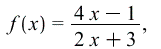 determine

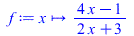 |
(4.1.1) |

 |
(4.1.2) |

 |
(4.1.3) |

 |
(4.1.4) |
As a check:

 |
(4.1.5) |
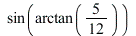
2. Assume 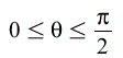 . Given
  , determine
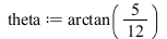
 |
(4.2.1) |

 |
(4.2.2) |
OR
 |
(4.2.3) |

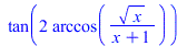
3. Assume  . Given
  , determine
  and
and 


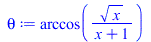 |
(4.3.1) |

 |
(4.3.2) |

 |
(4.3.3) |

 |
(4.3.4) |

 |
(4.3.5) |

 |
(4.3.6) |
4. Given 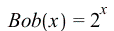 and
and  , determine:





 |
(4.4.1) |

 |
(4.4.2) |

 |
(4.4.3) |

 |
(4.4.4) |

 |
(4.4.5) |

 |
(4.4.6) |
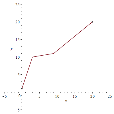
5. Define a piecewise function for the following image:


 |
(4.5.1) |


 |
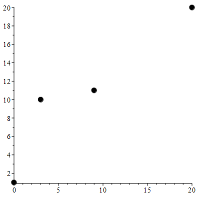
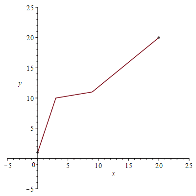
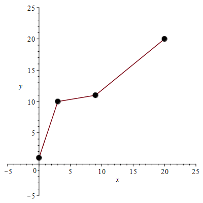
6. Recreate the image, with the points, in Maple.

![A := [0, 1]; 1; B := [3, 10]; 1; C := [9, 11]; 1; E := [20, 20]](images/Maple 19 SVDiff Calc Document Solutions_393.gif)
![A := [0, 1];](images/Maple 19 SVDiff Calc Document Solutions_394.gif) |
|
![B := [3, 10];](images/Maple 19 SVDiff Calc Document Solutions_395.gif) |
|
![C := [9, 11];](images/Maple 19 SVDiff Calc Document Solutions_396.gif) |
|
![E := [20, 20];](images/Maple 19 SVDiff Calc Document Solutions_397.gif) |
(4.6.1) |

![Pts := pointplot([A, B, C, E], symbolsize = 20, symbol = solidcircle);](images/Maple 19 SVDiff Calc Document Solutions_399.gif)
 |

 |

 |
7. Determine the inverse of the function. Do you notice anything interesting about the slope values?

![piecewise(`<`(x, 1.), [], `<=`(x, 10.), [`+`(`-`(.3333333333), `*`(.3333333333, `*`(x)))], `<=`(x, 11.), [`+`(`-`(57.), `*`(6., `*`(x)))], `<=`(x, 20.), [`+`(`-`(4.444444444), `*`(1.222222222, `*`(x))...](images/Maple 19 SVDiff Calc Document Solutions_406.gif) |
(4.7.1) |

![piecewise(`<`(x, 1), [], `<=`(x, 10), [`+`(`-`(`/`(1, 3)), `*`(`/`(1, 3), `*`(x)))], `<=`(x, 11), [`+`(`-`(57), `*`(6, `*`(x)))], `<=`(x, 20), [`+`(`-`(`/`(40, 9)), `*`(`/`(11, 9), `*`(x)))], `<`(20, ...](images/Maple 19 SVDiff Calc Document Solutions_408.gif) |
(4.7.2) |


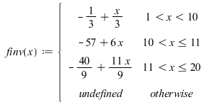
 |
(4.7.3) |




8. Plot the function and its inverse, and
 on the same image.
![plot([f(x), finv(x), x], x = -5 .. 20);](images/Maple 19 SVDiff Calc Document Solutions_419.gif)
 |
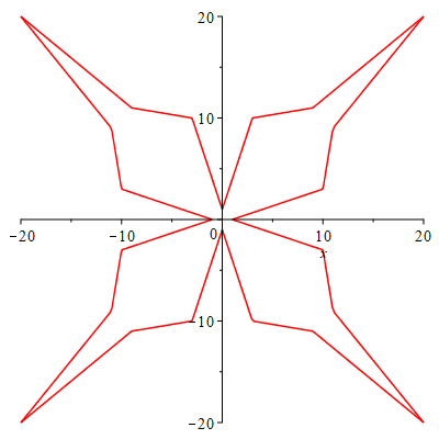
9. Use symmetry to plot the function and its inverse to create the following image: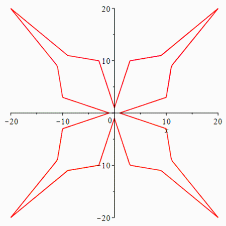
![plot([f(x), finv(x), `+`(`-`(f(x))), `+`(`-`(finv(x))), f(`+`(`-`(x))), `+`(`-`(f(`+`(`-`(x))))), finv(`+`(`-`(x))), `+`(`-`(finv(`+`(`-`(x)))))], x = -20 .. 20, color = red);](images/Maple 19 SVDiff Calc Document Solutions_422.gif)
 |